What Do 39 Popular Cannabis Strains Have in Common?

Published April 25, 2026 · Data sourced from GrowDiaries.com · Analysis by K-Means clustering with PCA dimensionality reduction

GrowDiaries surfaces a dense set of features per strain: THC and CBD percentages, flowering time, indica/sativa genetics, yield metrics, difficulty ratings, effects profiles, and community engagement stats. I wanted to see whether the data reveals natural groupings when you look at all features simultaneously rather than one at a time.

Contents

The Dataset
Methodology
Choosing k
PCA & Dimensionality Reduction
The Three Clusters
Cluster Profiles
Feature Distributions
Feature Correlations
Key Takeaways
Limitations & Next Steps

1. The Dataset

I scraped the top 40 strains from GrowDiaries’ strains page (the first page of results, sorted by popularity). One strain (Cereal Milk) was excluded due to a missing community rating—likely insufficient data on the platform—leaving 39 strains in the analysis.

Each strain came with 11 numeric features used for clustering:

Feature	Description	Range in Dataset
THC %	Advertised THC content	10–34%
CBD %	Advertised CBD content	0.05–1.4%
Flowering Days	Expected flowering period	57–100 days
Indica %	Genetic ratio (indica vs. sativa)	0–100%
Yield Weight (g)	Expected yield in grams	195–420g
Avg Rating	Community rating (0–10)	7.6–9.6
Avg Weight/Plant (g)	Actual harvested weight per plant	36–225g
Avg g/Watt	Yield efficiency (grams per watt of light)	0.23–0.86
Reviews	Number of community reviews	4–617
Harvests	Number of logged harvests	3–775
Growers	Number of unique growers	18–1362

All features were standardized (z-scored) before clustering to prevent high-magnitude features like grower count from dominating the distance calculations.

2. Methodology

The analysis pipeline was straightforward: standardize features with StandardScaler, apply K-Means clustering, and project the results into 2D using PCA (Principal Component Analysis) for visualization. K-Means was chosen for its interpretability and speed on small datasets. With only 39 observations and 11 features, more complex methods like DBSCAN or Gaussian Mixture Models would be overkill and harder to explain.

Scikit-learn’s implementation was used with n_init=30 (30 random initializations, keeping the best) to avoid convergence to local optima. Reproducibility was ensured with random_state=42.

3. Choosing k

The eternal question in K-Means: how many clusters? I evaluated k = 2 through 8 using two standard heuristics.

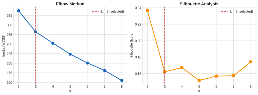
Figure 1. Elbow method (left) and silhouette analysis (right). The elbow flattens around k=3, and silhouette scores are modest across the board.

The elbow plot shows inertia (within-cluster sum of squares) decreasing as k increases, with diminishing returns visible around k = 3. The silhouette analysis peaks at k = 2 (score = 0.237) but k = 3 (score = 0.162) offers a more granular and interpretable grouping.

A note on silhouette scores: Values below 0.25 indicate overlapping clusters, which is expected here. Cannabis strains exist on a continuum, not in discrete categories. The clusters should be read as tendencies, not hard boundaries.

4. PCA & Dimensionality Reduction

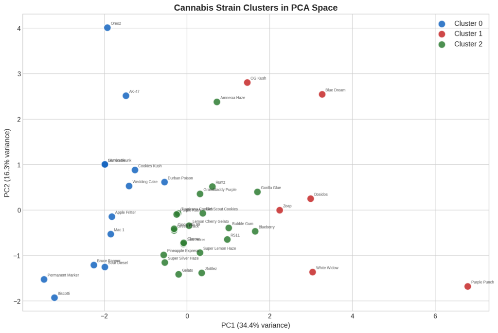
To visualize 11-dimensional data in 2D, I used PCA. The first two principal components capture 34.4% and 16.3% of the total variance respectively (50.7% combined). The 2D plot is a useful approximation but doesn’t tell the whole story.

Figure 2. PCA loading vectors. PC1 is driven primarily by community engagement metrics (reviews, harvests, growers). PC2 is driven by yield efficiency (g/watt) and yield weight vs. flowering days.

The loadings reveal that PC1 is essentially a “popularity” axis — strains with more reviews, harvests, and growers load strongly to the right. PC2 separates strains by growing efficiency: high g/watt and yield weight push strains upward, while longer flowering times push them downward. THC and CBD load moderately but in opposite directions, reflecting the well-known inverse relationship between cannabinoid concentrations.

5. The Three Clusters

Figure 3. All 39 strains projected onto the first two principal components, colored by cluster assignment.

Cluster 0 — “The Potent Boutiques” (13 strains)

Permanent Marker, Apple Fritter, Biscotti, Oreoz, Sour Diesel, Wedding Cake, Bruce Banner, Mac 1, Durban Poison, Cookies Kush, AK-47, Slurricane, and Lemon Skunk.

Highest average THC (23.5%), highest yields (318g), highest community ratings (8.94/10). Fewer growers (avg 83) and reviews (avg 33) — high-quality but less established on the platform. Difficulty skews harder: 7 rated “difficult,” 6 “moderate,” zero “easy.” Effects: relaxed, euphoric, creative. Flavors: sweet, earthy, diesel.

Cluster 1 — “The Proven Workhorses” (6 strains)

Zoap, Dosidos, OG Kush, Purple Punch, White Widow, and Blue Dream.

Smallest cluster, most distinctive. Highest community engagement by a wide margin: averaging 532 growers, 212 reviews, 274 harvests. Easiest to grow (4 of 6 rated “easy”), shortest flowering time (70 days), best yield efficiency (0.60 g/watt). Higher CBD (0.97%), more indica (62%). Effects lean sedative. These are the strains the community has actually validated at scale.

Cluster 2 — “The Balanced Mainstream” (20 strains)

Zkittlez, Gorilla Glue, Runtz, Granddaddy Purple, Lemon Cherry Gelato, Gelato, RS11, Tropicana Cookies, Blueberry, Girl Scout Cookies, Super Lemon Haze, Jack Herer, Amnesia Haze, Green Crack, Super Silver Haze, Pineapple Express, Cheese, Purple Kush, Bubble Gum, and Cinderella 99.

The largest cluster. Moderate THC (18.9%), moderate engagement (249 growers, 94 reviews), moderate yield (273g), balanced difficulty distribution. Well-known, broadly popular strains that don’t specialize in any extreme — the center of mass of the dataset.

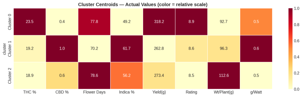
6. Cluster Profiles

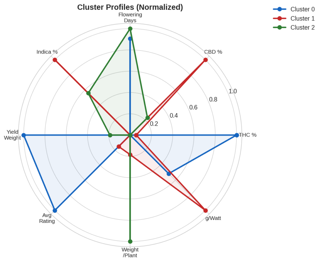
Figure 4. Normalized radar chart showing each cluster’s profile across 8 key features. Each axis is scaled 0–1 relative to the min/max across clusters.

Cluster 0 (blue) dominates on THC, yield weight, and rating, but trails on CBD and g/watt. Cluster 1 (red) leads on CBD, g/watt, and weight per plant, but has lower THC. Cluster 2 (green) is consistently in the middle.

Figure 5. Heatmap with actual centroid values annotated.

Cluster 1’s g/watt of 0.6 is 30% higher than Cluster 2’s 0.46 — meaningful for anyone watching electricity costs. Cluster 0’s 23.5% THC is 4.5 points above Cluster 2.

7. Feature Distributions

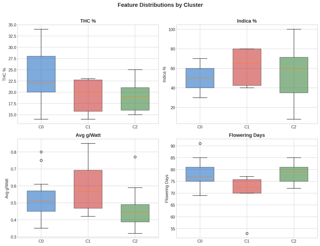
Figure 6. Box plots showing the distribution of four key features within each cluster.

Cluster 0’s THC distribution is right-shifted with Permanent Marker as a high outlier at 34%. Cluster 1 shows tight distributions across most metrics — similar in averages and in consistency. Cluster 2’s indica % has the widest spread, reflecting its catch-all nature: it contains both 100% sativas like Durban Poison and heavy indicas like Purple Kush.

8. Feature Correlations

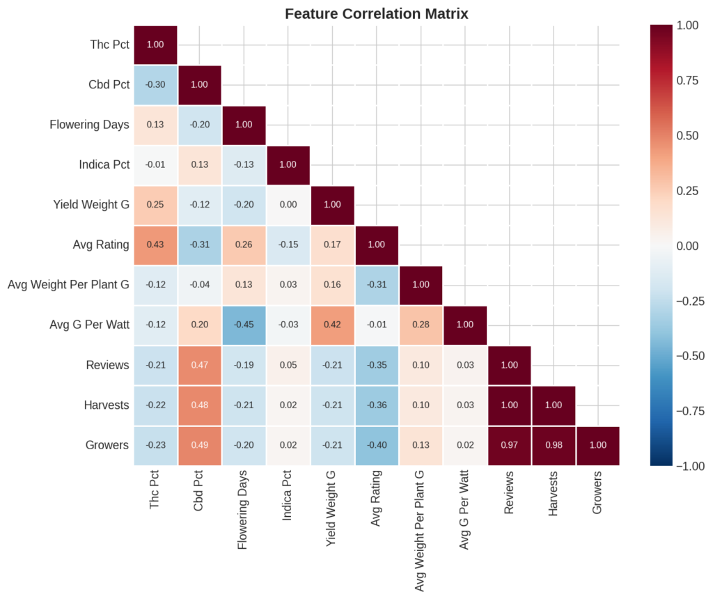
Figure 7. Pairwise Pearson correlations across all 11 features.

The three community engagement metrics (reviews, harvests, growers) are highly correlated with each other (r > 0.95) — they all measure platform popularity. CBD and THC show a moderate negative correlation (r ≈ −0.3), consistent with the cannabinoid synthesis pathway tending to favor one over the other. Avg g/watt correlates moderately with CBD (r ≈ 0.35).

9. Key Takeaways

Cluster 0 strains average 23.5% THC and 318g yields, but expect harder grows and less community documentation to lean on. Cluster 1 strains (OG Kush, White Widow, Blue Dream, etc.) have been grown by 500+ community members on average, flower fastest, and are the most light-efficient at 0.60 g/watt — four of six are rated “easy.” The moderate silhouette scores (0.16–0.24) confirm that strains exist on a continuum rather than in discrete buckets. The strongest separation axis is community engagement, not genetics — platform popularity may be as structurally important as biological traits in how strains cluster in real-world data.

10. Limitations & Next Steps

This covers only the top 40 strains from GrowDiaries’ first page. A larger sample would likely reveal more structure. The features mix biological attributes (THC, CBD, flowering time) with community metrics (reviews, growers), which operate on fundamentally different dynamics — a strain’s grower count reflects marketing and availability as much as genetics. Clustering on biological features alone, then overlaying community metrics for interpretation, would be more rigorous.

Hierarchical clustering might better capture nested structure, and DBSCAN could find density-based groupings without requiring a pre-specified k. Terpene profiles would likely improve cluster separation significantly — GrowDiaries doesn’t surface them in structured form.

These results also reflect a snapshot at the time of scraping. Community metrics shift as new growers discover strains, and THC % can vary between phenotypes of the same cultivar.

Tools used: Python 3, scikit-learn (KMeans, PCA, StandardScaler, silhouette_score), matplotlib, seaborn, pandas. Data sourced from GrowDiaries.com on April 25, 2026.